Morsels

These are "morsels" — little ideas or results that can be expressed in a short space. They may be exported or extended to full articles at a later time. (You can go to page 2)

1. Convex shadows. Any convex 3D object will have a silhouette of a certain area. Averaged over all viewing angles, the size of the silhouette is exactly a quarter of the object's surface area.

   Why? By dimensional analysis, the size of the silhouette must be proportional to surface area. By subdividing the surface into shadow-casting pieces, you can prove that the constant doesn't depend on shape as long as the shape is convex. So use the example of a unit sphere to compute its value.

   The same principle applies in higher dimensions \(n\). The formulas for sphere surface area and volume involve the gamma function, which simplifies if you consider odd and even dimensions separately. Let \(\lambda_n\) designate the constant for \(n\) dimensions. Then:

   \[\lambda_{n+1} = \begin{cases}\frac{1}{2^{n+1}} {n \choose n/2} & n\text{ even}\\\frac{1}{\pi}\frac{2^n}{n+1} {n \choose {\lfloor n/2\rfloor} }^{-1} & n\text{ odd}\end{cases}\]

   \[\lambda_n = \frac{1}{2},\; \frac{1}{\pi},\; \frac{1}{4},\; \frac{2}{3\pi},\; \frac{3}{16},\; \frac{8}{15\pi},\; \ldots .\]

2. M'aide!. One afternoon, you call all your friends to come visit you. If they all depart their houses at once, travel in straight lines towards you, and are uniformly distributed throughout the surrounding area, how many people should you expect to arrive as time goes by?

   The expected number of arrivals at each moment is proportional to the time since you called. Imagine a circle, centered on you, whose radius expands at the same rate everyone travels. Whenever the circle engulfs someone's house, that's the exact moment the person arrives at your door. Uniform distribution implies number of new arrivals proportional to circumference; number of cumulative arrivals proportional to area.

   Same principle generalizes to higher dimensions \(n\).

3. Connect infinity. Extend the board game connect four so that it has infinitely many columns. You win after infinitely many moves if you've constructed an unbroken rightwardly-infinite horizontal sequence of pieces in any row and your opponent hasn't. (You don't need to fill the whole row, and diagonal/vertical chains don't count in this game.) Prove that you can force a draw.

   Nailing down the proof is subtle, because blocking strategies for lower rows don't always generalize to higher rows. The general principle is to block your opponent infinitely many times in each row, preventing an unbroken chain. The specific principle is: to stop your opponent from reaching height \(k\) in a certain column, don't put any pieces there; wait until they build a tower of height \(k-1\) then put your piece on top.

   For each row, choose infinite disjoint subsets of \(\mathbb{N}\): \(T_1, T_2, T_3, T_4\). Each \(T_k\) is a predetermined list of columns where you will interrupt your opponent's towers of height \(k\). Whenever your opponent moves, if their piece builds a tower of height \(k-1\) in a column in \(T_k\), put your next piece on top. Otherwise, put your piece in an empty column of \(T_1\) to the right of all pieces played so far.

   You never put pieces on your opponent's except to block them, and this blocking process cannot be stopped. A key insight is you can't stymie your opponent by building your own interrupting towers, only by stopping theirs. There is no way to build a tower of height 3 or 4 if the other player wants to prevent it.

4. Blackout Turing machines. A "blackout machine" is a Turing machine where every transition prints a 1 on the tape. The halting problem for blackout machines is decideable.

   The tape of a blackout machine always consists of a contiguous region of 1s surrounded by infinite blank space on the left and right. Any machine that reads sufficiently many ones in a row must enter a control loop. By measuring the net movement during the loop, you can decide whether the machine will overall go left, right, or stay in place each iteration. Regardless of how many ones are in a row, using modular arithmetic, you can efficiently predict what state the machine will be in when it exits.

   By this reasoning, a state-space graph will help us fast-forward the looping behavior of the machine. A q-state machine can enter a loop with period 1, 2, 3, …, or at most q. To anticipate its behavior on any-sized string of ones, it's therefore enough to know what the string size is mod 2, mod 3, …, mod q. Thus, for each option of left-side/right-side, each possible state of the machine's control, and each possible value of string length mod 2, mod 3, mod 4,… mod q, the graph has a node. By simulating the machine, you can efficiently compute the transitions between nodes of this graph, recording how the machine-and-tape will look whenever the machine exits the string of ones. (Add a special node for "loops forever within the string of ones" and "halts").

   There are (on the order of) q! nodes in this graph—overkill, but still finite. You can simulate the machine in fast-forward using these graph transitions. After simulating a number of transitions equal to the number of nodes in this graph, the machine must either halt, loop forever within the region of ones, or revisit a node (in which case it loops forever, growing the region of ones).

5. Lopped polygons. Lop off the edges of a regular polygon, forming a regular polygon with twice as many edges. Repeat this process until, in the limit, you obtain a circle. As you might expect, that circle turns out to be the incircle of the polygon (i.e. the largest circle contained in it).

   Interestingly, the cutting process multiplies the original perimeter of the object by \((\pi/n) \cot(\pi/n)\), where \(n\) is the original number of sides. It multiples the area by the same amount (!).

6. NP-complete morphemes. If you have a language (set) of even length strings, you can form a language comprising just the first half of each string, or just the second half.

   1. Is there a language which is in P, but where each half-language is NP-complete?
   2. Is there a language which is NP-complete, but where each half-language is in P?

   (What are P and NP?¹)

   The answer to both questions is yes. For the first question, make a language of strings where each half contains a hard problem and a solution to the problem in the other half. Then each half-language is hard because it's a hard problem paired with a solution to an unrelated problem. But the combined language is easy because then both problems come with solutions.

   For the second question, make a language by pairing up easy problems according to a complicated criterion. So the half-langauges are easy, because they're just sets of easy problems. But the overall language is hard because deciding whether the pairing is valid is hard.

   Concrete examples: In the first question, take strings of the form GxHy, where G and H are isomorphic Hamiltonian graphs; x is a Hamiltonian path through H; and y is an isomorphism from G to H. (Pad as necessary so Gx and Hy have the same length.) When Gx and Hy are separated, the strings x and y provide no useful information, so each half-language is as hard as HAMPATH. When united, GxHy is easy because x and y easily allow you to confirm that G and H are Hamiltonian.

   In the second question, take strings of the form GH where G and H are graphs and G is isomorphic to a subgraph of H. This is an NP-complete problem. But each half-language is just the set of well-formed graphs, which is easy to check.

7. Juking jukebox. I couldn't tell whether my music player was shuffling songs or playing them in a fixed sequential order starting from the same first song each session. Part of the problem was that I didn't know how many songs were in the playlist, and all I could retain about songs is whether I had heard them before (not, e.g., which songs usually follow which).

   You can model this situation as a model-selection problem over bitstrings representing whether played songs have been heard (0) or not-heard (1). Every bitstring is consistent with random play order, but only a handful are consistent with sequential play order (...0001111...). Therefore, the longer you listen and remain unsure, the vastly more probable the sequential model is. (Specifically if you play n songs, there are n+1 outcomes consistent with sequential play out of 2ⁿ total outcomes.) (And yes; turns out my music player was sequential, which was strongly indicated by the fact that I felt unsure it was random in the first place.)

8. Loop counting. If there's a unique two-step path between every pair of nodes in a directed graph, then every node has \(k\) neighbors and the graph has \(k\) loops, where \(k^2\) is the number of nodes in the graph.

   

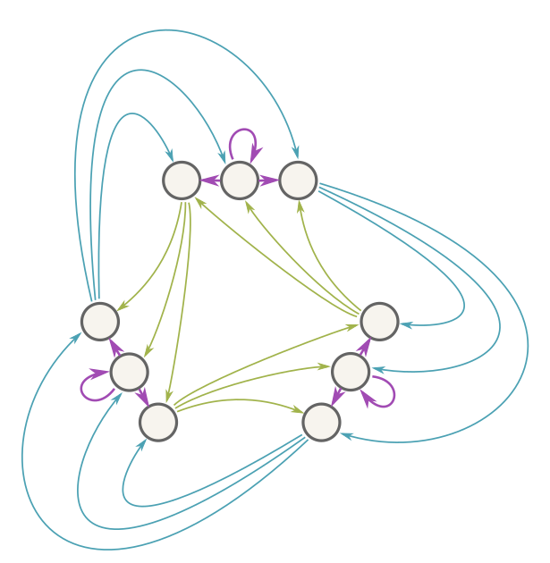
   Astonishingly, you can prove this result using the machinery of linear algebra. You represent the graph as a matrix \(M\) whose \((i,j)\) entry is one if nodes \(i\) and \(j\) are neighbors, or 0 otherwise. The sum of the diagonal entries (the trace of the matrix) tells you the number of loops. The trace is also equal to the sum of the generalized eigenvalues, counting repetitions, so you can count loops in a graph by finding all the eigenvalues of the corresponding matrix.

   The property about paths translates into the matrix equation \(M^2 = J\), where \(J\) is a matrix of all ones. (The r-th power of a matrix counts r-step paths between nodes.) This matrix \(J\) has a number of special properties—multiplying a matrix by \(J\) computes its row/column totals (i.e. the number of neighbors for a graph!), multiplying \(J\) by \(J\) produces a scalar multiple of \(J\), and \(J\) zeroes-out any vector whose entries sum to zero; this is an \(n-1\) dimensional subspace. The property that \(M^2=J\), along with special properties of \(J\), allows you to conclude that higher powers of \(M\) are all just multiples of \(J\); in particular, examining \(M^3=MJ=JM\) reveals that every node in the graph has the same number of neighbors \(k\). So \(M^3 = kJ\). (And \(k^2 = n\) because \(k^2\) is the number of two-step paths, which lead uniquely to each node in the graph.) Notice that because of this neighbor property, \(M\) sends a column vector of all ones to a column vector of all k's, so \(M\) has an eigenvalue \(k\). Based on the powers of \(M\), \(M\) furthermore has \((n-1)\) generalized eigenvectors with eigenvalue zero. There are always exactly \(n\) independent generalized eigenvalues, and we've just found all of them. Their sum is \(0+0+0+\ldots+0+k = k\), which establishes the result.

   The same procedure establishes a more general result: If there's a unique r-step path between every pair of nodes in a graph, then every node has \(k\) neighbors and the graph has \(k\) loops, where \(k^r\) is the number of nodes in the graph.

9. Cheap numbers. The buttons on your postfix-notation calculator each come with a cost. You can push any operator (plus, minus, times, floored division, modulo, and copy) onto the stack for a cost of one. You can also push any integer (say, in a fixed range 1…9) onto the stack; the cost is the value of the integer itself. Find the smallest-cost program for producing any integer.

   For example, optimal programs for the first few integers are 1, 2, 3, 2@+, 5, 3@+, 13@++, 2@@**, 3@*. (Here @ denotes the operator which puts a copy of the top element of the stack onto the stack.)

   You can find short programs using branch-and-bound search to search the space of stack states. There are some optimizations: Using dynamic programming (Dijkstra's algorithm), you can cache the lowest-cost path to each state so that you never have to expand a state more than once. Second, you can use the size of the stack state as an admissible heuristic: if a stack has \(n\) items in it, it will take at least \(n-1\) binary operators to collapse it into single number.

   There's a nice theorem, too: For any integer, the lowest-cost program only ever needs the constants 1 through 5 (additional constants never offer additional savings). The program never costs more than the integer itself, and in fact for sufficiently large integers (over 34), it costs less than half of the integer.

   To prove the theorem, first show that every integer \(n\) has a (possibly nonoptimal) program which costs at most \(n\) and which uses the constants 1…5 ². Next, suppose you have an optimal-cost program which uses any set of constants. By the previous result, you can replace each constant with a short script that uses only 1…5, and this substitution won't increase the program's cost. Hence the program-with-substitutions is still optimal, but only uses the digits 1…5, QED.

10. Rolls with Advantage. In D&D5e, certain die rolls have advantage, meaning that instead of rolling the die once, you roll it twice and use the larger result. Similarly, a modifier is a constant you add to the result of a die roll. There's a simple probabilities nomogram for deciding whether you should prefer to roll (d20 + x) with advantage, or (d20 + y).

    

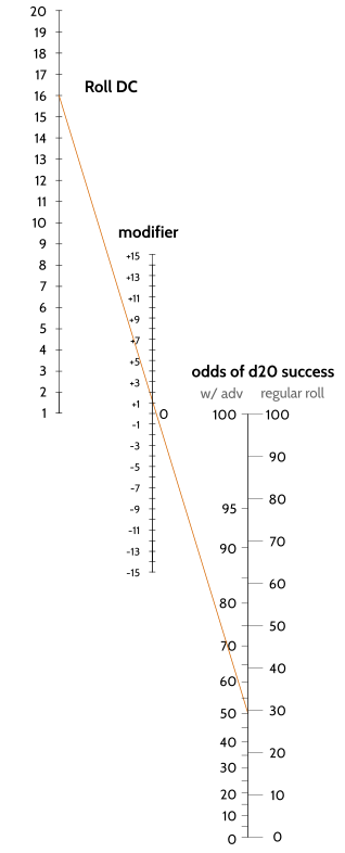
    To use: draw a line from the DC on the first axis to the modifier on the second axis and continue until you hit the third axis. Read the right-hand value for the probability of success when rolling d20, or the left hand value when rolling d20 with advantage. For example, the orange line shows a situation where DC=16, modifier=+1. With advantage, success rate is around 50%. Without, it's around 30%.

    The equation governing the odds \(P\) of beating a DC of \(D\) with a modifier of \(X\) when rolling a g-sided die is: \[g (1-P) = (1-D+X) \]

    With advantage, the equation is surprisingly similar: \[g \sqrt{(1-P)} = (1-D+X) \]

    And so both can be plotted on the same sum nomogram.

11. Categorical orientations. The pan and ace orientations are optimal in a certain mathematically rigorous sense. They factor out gender (in the definition, you don't need to know the person's gender or the person's model of gender), and they form what is called a categorical adjunction or Galois connection:

    Consider the space of possible orientations. If we assume that each person has exactly one gender and that an orientation comprises a subset of attractive genders, then the space of possible orientations becomes a set \(G \times 2^G\). We can equip \(2^G\) with subset ordering; because genders aren't ordered, we'll equip \(G\) with the identity order (each gender is comparable only to itself). \(G\times 2^G\) has the induced product order.

    There is a disorientation functor \(\mathscr{U}:G\times 2^G\rightarrow G\) which forgets a person's orientation but not their gender. Observe that the left adjoint of \(\mathscr{U}\) assigns an ace orientation to each person: \(g\mapsto \langle g, \emptyset\rangle\). And the right adjoint of \(\mathscr{U}\) assigns the pan orientation to each person: \(g\mapsto \langle g, G\rangle\). Each one represents a certain optimally unassuming solution to recovering an unknown orientation³.

    \[\mathbf{Ace} \vdash \mathbf{Disorient} \vdash \mathbf{Pan}\]

    P.S. The evaluation map \(\epsilon\) ("apply") detects same-gender attraction: In programming, evaluation sends arguments \(\langle f, x\rangle\) to \(f(x)\). Every subset of \(G\) is [equivalent to] a characteristic function \(G\rightarrow \{\text{true}, \text{false}\}\). So if we apply eval to an orientation in \(G\times 2^G\), we determine whether it includes same-gender attraction.

12. Geometric orientations. There is a vast potential for amusing orientation-based results in differential geometry, which is a subject I don't yet have the expertise to formalize. For example, if you conceive of a manifold of possible genders with a designated base point for one's own gender, then you can define attraction to a gender by the existence of a geodesic joining them (orientation assigns an overall shape to the gender manifold); closed geodesics, indicative of same-gender attraction, exist only in the presence of curvature and therefore imply that the manifold is not flat.

13. Pyramid puzzles The objective of the number-tower puzzle is to fill in numbers in a triangular structure so that every number is equal to the sum of the two numbers below it. Some numbers are specified in advance, providing constraint. Example:

    

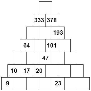
    The question is, when designing such a puzzle, how many and which spaces should you specify in advance to guarantee that there is a single unique solution? For example, specifying all values at the base nodes is sufficient. How do you characterize all such arrangements?

    Solution: Let \(h\) be the height of the tower. If you place \(h\) values in the tower such that you can't solve for any one value in terms of the others, then those \(h\) values uniquely determine a solution. You never require more or less than \(h\) values.

    You can prove this using methods of linear algebra. The addition constraints for the tower define a system of linear equations (\(x_1 + x_2 = x_3\), and so on), which you can represent as a matrix. Because filling out the \(h\) base nodes of the tower uniquely determines the solution, and because the problem is linear, it always takes \(h\) independent values to determine a solution.

    You can formalize the "solve for one value in terms of the other" in terms of a matrix determinant. Construct the ancestral path matrix \(N\) with one column for every node, and one row for every node specifically in the tower base. In each entry, put the number of distinct upward paths to that node from that base node. Next, if you choose \(h\) tower positions to fill in, pick out the corresponding columns of \(N\) and combine them into an \(h\times h\) matrix, \(D\). Those \(h\) positions uniquely determine the entire pyramid if and only if \(D\) is invertible, i.e. has a nonzero determinant.

    This is because the rows of the ancestral path matrix \(N\) span the solution space—each row is a primitive solution. \(N\) sends the \(h\) parameters of the solution space to a complete filled-out solution. Selecting \(h\) columns of \(N\) amounts to forgetting (quotienting out) all but the \(h\) filled-in values in the complete solution. If you can undo the forgetting effect of $D$—if you can recover the \(h\) parameters of the solution space (e.g. the base tower values) from the filled-in values—then you can uniquely determine the complete solution from the filled in values.

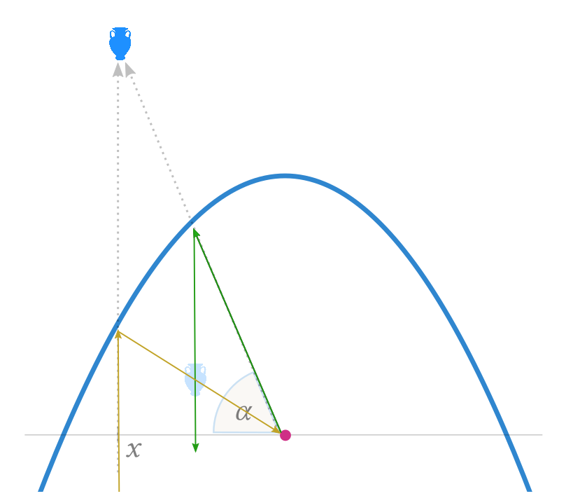
14. Charting the mirror world. A parabolic mirror distorts shapes in the real world. By creating strange anti-distorted shapes, you can create shapes whose reflections "in the mirror world" look normal. With the right coordinate system, the anti-distortion transformation has surprisingly simple form. It's:

    \[\widehat{x} = \frac{1 + \sin{\alpha}}{\cos{\alpha}}\] \[\widehat{\alpha} = \frac{1/4x^2 - f}{x}\]

    Here (see figure), the parabola's focus is at the origin, the $x$-axis is perpendicular to the optical axis, and the angles \(\alpha\) are measured relative to the origin and x-axis. Every point, real or virtual, is uniquely defined by an \(\langle x, \alpha\rangle\) pair. Parabolas characteristically reflect vertical rays into rays through the focus and vice-versa; this is how you prove the above transformation, and why the transformed \(\widehat x\) coordinate is defined purely in terms of the original angle \(\alpha\) and vice-versa.

    Miraculously, even in 3D these anti-distorted figures will have reflections that look correct from any viewing angle (!).

    I imagine you could do this same trick for mirrors shaped like other conic sections (ellipse, hyperbola) but I haven't tried yet.

    

15. Adjunctions as rounding. (A fun math fact.)

    There is a map \(i:\mathbb{N}\hookrightarrow \mathbb{R}\) which includes the natural numbers into the reals (by "typecasting"). Considering \(\mathbb{N}\) and \(\mathbb{R}\) as poset categories, the inclusion has both a left adjoint and a right adjoint.

    As you can guess, they're the floor and ceiling functions: if the floor of a number is at least \(n\), then the number itself is at least \(n\), and conversely. This makes floor, perhaps surprisingly, the right adjoint.

    \[\lceil \rceil\;\; \vdash \;\; i \vdash \;\; \lfloor \rfloor\]

    At least spiritually, an adjunction is exactly like this: the left adjoints round up, adding additional structure, while the right adjoints round down, forgetting it.

16. Sundial curves. The shadow cast by the tip of a sundial always traces out a conic section. There is a cone formed by the daily circular path of the sun and the tip of the sundial. The shape changes with latitude and season; depending on whether the sun rises and sets (hyperbola), always stays above the horizon (ellipse), or just grazes the horizon (parabola).

    Click the image below to see the animation.

    

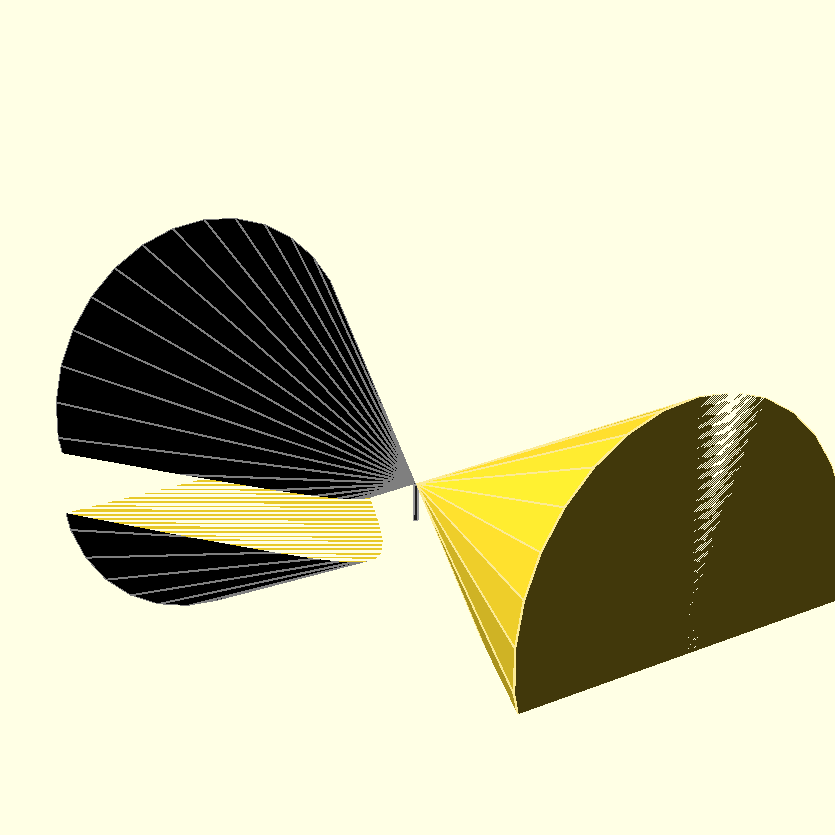
    The base of the golden cone shows the daily circular path of the sun. The tip of the gnomon casts a shadow where the black cone intersects the ground. In the animation, the cones tilt as you change latitudes, and the shadow changes from hyperbolic to elliptical.

17. Rainbow materials. A rainbow is formed at the boundary between two materials that bend light differently, such as water and air. Rainbows form perfect circles whose center is in the shadow of your head (the antisolar point) and whose size is determined by the two light-bending materials, irrespective of where you are.

    For example, when it rains on the ocean, a rainbow formed from the salty sea spray will have a smaller extent than a rainbow formed from falling rainwater. This is because salt water bends light differently than pure water.

    You can use the laws of optics to compute the rainbow's angular extent based on the materials involved ⁴. I have plotted the relationship in the chart below. As far as I have found, this is the first chart ever to depict rainbow size for materials other than water (which forms rainbows approximately of size 42.5° in air.)

    

    “Rainbow arc nomogram” by Dylan Holmes can be reused under the CC BY-SA license.

18. Visual clocks. A clock's two hands move as shown in the picture below:

    

    Using this kind of picture, you can visually find the twelve times (once per hour) that the positions of the hour and minute hand coincide (see where the red diagonal intersects the black trajectory):

    

    And you can answer more complicated questions, such as when you swap the positions of the hour and minute hands, how often is the result a valid configuration? ⁵ Indeed, swapping the hands means flipping the axes:

    

    And the swapped result is valid wherever it intersects the original graph, which it does in 12 x 12 - 1 = 143 distinct places:

    

19. Algebraic blood typing. The Jewish dietary law prohibiting mixtures of meat and milk has the same algebraic structure as the rules for which blood types are compatible donors—if you know one set of rules, you can transfer to the other.

    In Jewish law, food is categorized by whether it contains meat, dairy, both, or neither, with some strict observers using color-coded dishware for each category⁶. Note that if you start with food of one type and mix in some other food, you might change its category (e.g. from containing only meat to containing both meat and dairy), contaminating the dishware.

    In the simple ABO blood typing model, blood is categorized by whether it has A antigens, B antigens, both or neither. (Blood with both is called type AB; blood with neither is called type O.) To avoid an adverse clotting reaction, the donation rule is that blood with a particular antigen cannot be donated to blood without it.

    The dietary laws and blood-typing laws are algebraically the same: food containing meat or milk is analogous to blood expressing A or B antigens. If you mix a little food into your main food, you may contaminate the dishware. If you donate a little blood to a person, the result may cause blood clotting. Contaminated dishware and blood clotting happen under equivalent circumstances.

    Now you can determine that Type O blood is the universal donor, analogous to parev food (without meat or dairy). AB is the universal recipient, analogous to basar bechalav food (with both meat and dairy).

    Meat-only and dairy-only foods are like type A and type B blood. Accordingly, A can donate to A or AB, and can receive from A or O. Similarly, basari food can be mixed into a dish of basari or basar bechalav food without affecting the dish's category; and the basari category of a dish is unaffected if you mix in basari or parev food.

    ABO blood typing	Jewish dietary law
    Blood has A antigens, B antigens, both, or neither.	Food contains meat, milk, both, or neither.
    Type O blood has neither antigen.	Parev food has neither meat nor milk.
    Type AB blood has both antigens.	Basar bechalav food has both meat and milk.
    Donating some blood to a person can cause an adverse clotting reaction.	Mixing in a small amount of food can alter the category (meat/milk/both/neither) of a dish.

20. Conic conversions. The conic sections are a family of 2D shapes comprising hyperbolas, ellipses/circles, and parabolas. You can transform any conic section into any other using a projective transformation ("homography"). If you represent the shape using homogeneous coordinates, a homography is just an invertible 3x3 matrix.

    To transform the hyperbola \(y=1/x\) into the parabola \(y=x^2\), use: \(\mathbf{J}\equiv \begin{bmatrix}0&0&1\\0&1&0\\1&0&0\end{bmatrix}.\)

    To transform the hyperbola \(y=1/x\) into the ellipse \(x^2+y^2=1\), use: \(\mathbf{K}\equiv \begin{bmatrix}1&-1&0\\0&0&2\\1&1&0\end{bmatrix}.\)

    These matrices are invertible. By inverting, composing, scaling, translating, and rotating these transformations, you can therefore turn any conic into any other. (For example, to transform the standard parabola into the standard ellipse, use \(\mathbf{K}\mathbf{J^{-1}}\).)

21. Tunnel through the Earth. Suppose you magically construct a tunnel through the center of the Earth (ignoring heat, pressure, air friction, and a lot of other practical factors.) If you were to drop an object down the tunnel, it would fall until it reached the other side (accelerating as it approached the center of the Earth, then decelerating to a standstill as it reached the other side), then reverse direction and return to you, and so on.

    This is periodic motion, like an elastic spring or a pendulum or an orbit. You can use Newton's law of gravitation to find the force on the object as it falls. (The force turns out to be proportional to its distance from the center, just like with an ideal elastic spring.) The period of a round trip is around 5068 sec (84.5 min, \(T = 2\pi \sqrt{R_{\mathsf{Earth}} / g}\)), which means the object would pass through the Earth in around 42 minutes.

    Interestingly, the time period (84.5 minutes) is independent of a large number of factors. The tunnel can follow a diameter through the center of the Earth or any other chord. The tunnel can begin at the surface of the Earth or somewhere beneath it. (These variations are analogous to the way an elastic spring's period does not depend on how far it was stretched initially, or in which direction.)

    For similar reasons, a satellite in circular orbit very close to the surface of the Earth also travels periodically with the same period of 84.5 min. If the satellite were directly over the tunnel as you dropped an object down it, they would both reach the other side of the planet at the same time.

22. Netwonian insight A parabola is an ellipse with one focus at infinity. Closed orbits—such as a satellite orbiting the earth—are ellipse-shaped with one focus at the center of the earth⁷. For near-earth projectiles, the center of the earth is effectively infinitely distant. This is a geometric way to understand why near-earth projectiles seem to follow parabolic paths.

23. Calculus is small arithmetic. What if we invented a new positive number \(\delta > 0\) that was so small its square was zero (\(\delta^2 = 0\))?

    We'd get two complementary sets of numbers: ordinary-sized numbers like 1, 2, 3, and small numbers like \(\delta, 2\delta, 3\delta\). We can do arithmetic combining them together, like \(3+2\delta\) or \(\delta(4+7\delta)\). This numerical system is called dual numbers. Every number in this system has a ordinary-sized component and a small-sized component, just like complex numbers have real and imaginary components. They can all be written \(a + b\delta\).

    The surprise is that you can do calculus just using arithmetic with these dual numbers. For example, take any polynomial \(P(x)\) and apply it to a dual number \(a+b\delta\). Using the smallness property \(\delta^2=0\), you can prove that \(P(a+b\delta)\) is a dual number whose ordinary-sized part is \(P(a)\) and whose small part is the derivative \(b\cdot P^\prime(a)\) (!)⁸. Thus dual numbers give you a way to compute the derivatives of polynomials just by evaluating them.

    You can retrofit all smooth functions to work with dual numbers; just take this polynomial property as a definition for how ordinary functions should behave:

    \[f(a + b\delta) \equiv f(a) + (b\delta) \cdot f^\prime(a)\]

    With this definition, you can prove all of the differentiation rules from calculus using only arithmetic. For example, here's the product rule: If \(h(x) = f(x)g(x)\) then:

    \begin{align*} h(x+\delta) &= f(x+\delta)g(x+\delta)\\ & = [f(x) + \delta f^\prime(x)][g(x) + \delta g^\prime(x)]\\ & = f(x)g(x) + \delta \left[f^\prime(x)g(x) + f(x)g^\prime(x)\right] + \delta^2 [f^\prime(x)g^\prime(x)]\\ & = f(x)g(x) + \delta \left[f^\prime(x)g(x) + f(x)g^\prime(x)\right]\\ \end{align*}

    The small part of \(h(x+\delta)\) is \(h^\prime(x)\) by definition, and we have shown that this part is equal to \(f^\prime(x)g(x) + f(x)g^\prime(x)\), proving the product rule. As an exercise, you can prove the other differentiation rules (sum rule, chain rule, quotient rule⁹, etc.)

    These dual numbers are not just a mathematical curiosity; you can define them as a new datatype in a programming language. By defining a few primitive functions that use dual numbers, e.g. \(\sin(a+b\delta)\equiv \sin(a)+b\delta\,\cos(a)\), the definition above gives you a method for computing exact (not approximate) values for the derivative of any combination of those primitive functions. This is called automatic differentiation; it has practical applications in areas such as machine learning.

24. Conic number systems. The complex numbers introduce a special new number \(i\) with \(i^2=-1\). What would happen if you introduce \(j\) where \(j^2\) is some other real number?

    Such numbers still have "real" and "imaginary" components that combine separately. \((a+bj)+(c+dj)=(a+c) + j(b+d)\). You can make complex conjugates \(a+bj \leftrightarrow a-bj\). You can represent these numbers \((a+bj)\) using matrices of the form \(\begin{bmatrix}a & bj^2 \\ b & a\end{bmatrix}\), in which case matrix arithmetic (addition, multiplication, etc.) does the right thing.

    You can do arithmetic with these numbers, so you can form polynomials with them, so you can define the exponential as an infinite polynomial: \(\exp(jx) \equiv \sum_{k=0}^\infty \frac{(jx)^k}{k!}\). The "real" part of \(\exp{jx}\) comes from the even-numbered terms in the sum and behaves like cosine. The "imaginary" part comes from the odd-numbered terms and behaves like sine.

    Value of j2	Simplify \(\exp(jx)\)	Solve \((a+bj)(a-bj)=1\)	System name
    j2 = -1	\(\cos(x)\;+\; j\sin(x)\)	circle: a2 +b2 = 1	Complex numbers
    j2 = 0	\(1 \;+\; jx\)	two parallel lines: a2 = 1	Dual numbers
    j2 = +1	\(\cosh(x)\;+\;j\sinh(x)\)	hyperbola: a2 - b2 = 1	Split-complex numbers

    Multiplying a point by \(\exp{j\theta}\) moves that point along a circle ("rotation"), along two parallel lines ("translation"), or along a hyperbola ("hyperbolic rotation").

    If the real axis is space and the \(j\) axis is time, then these movements have a physical interpretation.

    Value of j2	Time is …	\(\exp{j\theta}\)	Change in reference frame
    j2 = -1	Spatial	Rotation	Rotate spatial axis
    j2 = 0	Classical	Translation	Galilean boost
    j2 = +1	Relativistic	Hyperbolic rotation	Lorenz boost

    Time is relativistic when \(j^2=+1\); the movement is a "Lorenz boost", changing from one person's spacetime coordinates to another. Time is classical when \(j^2 = 0\); the movement is a Galilean boost (\(\widehat{x} = x - vt\)). Time is just another dimension of space when \(j^2=-1\); the movement is a rotation in space-time. In all three cases, you can think of \(j^2\) as \(1/c\), the speed of light.

25. Birthdays and bitstrings. Suppose you assign a random k-bit identification number to \(n\) objects. What's the probability of a collision—that at least two objects are assigned the same id?

    If you plot the collision probability as a function of the number of bits \(k\), the curve is surprisingly S-shaped—nearly 100% when \(k\) is small, until it suddenly plunges, with a surprisingly graceful tail end, toward a 0% asymptote. Here, I've plotted the probability of collision if you randomly assign a k-bit id to each of the 100 bil neurons (\(n=10^{11}\)) in the human brain:

    

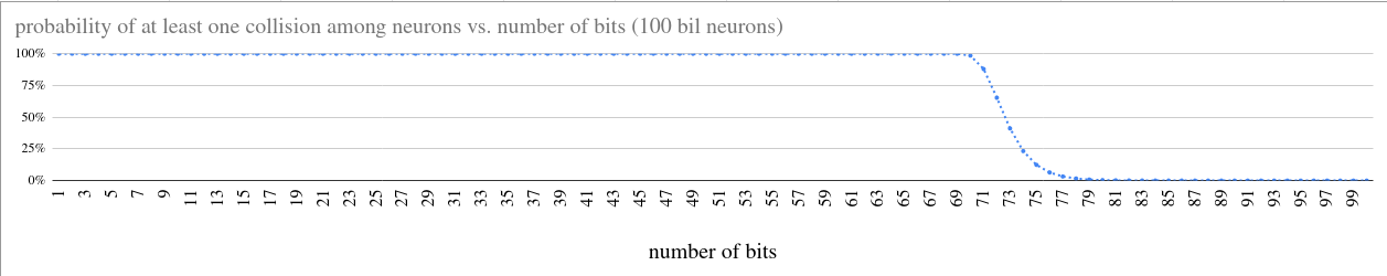
    I approximate the probability of birthday collision very closely as \(p(n,k) \approx 1-\exp(n(n-1)/2^{k+1})\), using the fact that \((1-x) \approx \exp(-x)\) whenever \(x\ll 1\).

    We can mark that steep transition between nearly 100% and nearly 0% by finding the place where the function changes most rapidly. This occurs when the numerator \(n(n-1)\) and denominator \(2^{k+1}\) are equal. Intuitively, this is when there is exactly one bitstring for every distinct pair of objects \(n(n-1)/2\) –in this specific case (n=100 bil neurons), when each bitstring has \(k\approx \mathbf{72}\) bits, corresponding to the \(n(n-1)/2 \approx 10^{22}\) possible pairs of neurons.

    Note that this is twice as many bits as you'd need if you were sequentially numbering the neurons by hand— \(\log_2(n)\) bits —rather than choosing numerical ids at random — \(\log_2( n(n-1)/2)\) bits. Concretely, if you were using hexadecimal strings as ids for neurons, you could use strings like 60 f4 51 ce ad for sequential numbering, but would need strings at least twice as long (20 49 3e 99 18 ab ac db 4d | b0 fd fa ce 56 f0 61 6f 5a) to comfortably avoid collisions when choosing at random.

26. Reading the pinhole camera. Suppose an ideal pinhole camera sits axis-aligned at the origin, pointing in the Z direction. Every homography (3x3 invertible matrix) describes how a particular plane in 3D space is transformed from world space into (homogeneous) 2D camera-screen space.

    In particular, the first two columns of the homography describe two 3D vectors (S,T) embeded in that plane, and the third column describes the plane's origin point U. Every point on that plane can be described as Sx + Ty + U. The point at Sx + Ty + U is projected onto the homogeneous point \(\begin{bmatrix}\vec{\mathbf{S}} & \vec{\mathbf{T}} & \vec{\mathbf{U}}\end{bmatrix}\cdot \begin{bmatrix}x&y&1\end{bmatrix}^\top\) on the camera's projection screen.

    Reading homographies this way provides a deeper understanding of Morsel #20 (Conic conversions): through foreshortening, you can make ellipses, hyperbolas, or parabolas, look like one another (or, really, segments of one another) when viewed through a pinhole camera. The homography tells you how to arrange a planar drawing of one conic so it looks like another.

    Bonus: because homographies are invertible and composable, it follows that you can transform between any two pinhole camera views of a common scene using a homography: send one view to a common plane, then send that plane to the other view.

27. An easier quadratic formula. (Loh's method). The goal is to factor the equation \[x^2 + bx + c = 0\] into \((x-r_1)(x-r_2)\) to expose the roots \(r_1, r_2\). By expanding, note that the roots have the key property that their sum is \(-b\) and their product is \(c\). In the usual guess-and-check method, you consider various ways of factoring \(c\) and check whether the sum is equal to \(-b\).

    In the new method, you use these properties to solve for the roots directly. You don't have to memorize the quadratic formula or make any guesses. Note that the midpoint (average) between the two roots is \(-b/2\), and the two roots lie equidistant from that midpoint. Given that the roots must have the form \(-b/2 \pm u\) for some unknown \(u\), their product is \((-b/2+u)(-b/2-u) = b^2/4 - u^2\). As noted, the product of the roots is also equal to \(c\). Hence we have an equation \(b^2/4 - u^2 = c\) that can be solved immediately for the unknown \(u\) just by addition and taking a square root. The roots are then \(r_i = -b/2 \pm u\).

    For example, in the equation \(x^2 + 8x - 9\), the roots are equidistant from -8/2 = -4. The product of the roots is \((-4-u)(-4+u) = 9\), which simplifies to \(16-u^2 = -9\). We solve for \(u\): \(u^2 = 25\), so \(u=5\). The two roots are \(-4 \pm 5\), i.e. 1 and -9. The overall factorization is \((x-1)(x+9) = x^2 +8x - 9\).

28. Random song access. The first song in your 100-song playlist is your favorite. Your music player has only two buttons: PREV (which goes to the previous song in the list) and RANDOM (which goes to a random song in the list, possibly the same one you're currently on). What's the ideal button-pressing strategy to get to your favorite song in as few presses as possible?

    Solution: Let's generalize to \(n\) songs.

    1. Because RANDOM wipes out PREV's progress, an ideal strategy will perform all the RANDOM presses before all the PREV presses. Whether PREV or RANDOM is better depends on where you are in the list.
    2. If you're sufficiently close to the start of the list, the optimal strategy is to press PREV repeatedly until you get to the start and win. Hence if you're not sufficiently close, the optimal strategy is to press RANDOM repeatedly until you become sufficiently close, then press PREV repeatedly until you win.

    3. We can solve for the precise value of "sufficiently close": Number the songs starting from 0, and let \(Z\) denote the last position where the PREV strategy is better than the RANDOM strategy.

       The PREV strategy takes exactly \(q\) steps, where \(q\) is your position in the list. The RANDOM strategy takes expected \(n/(Z+1) + Z/2\) steps. (Expected number of RANDOMs to get sufficiently close, plus expected number of PREVs to complete.)

       If \(Z\) is the last position where PREV is better than RANDOM, then \(Z\) must be the largest integer such that \(Z < n/(Z+1) + Z/2,\) i.e. such that

       \[\frac{Z(Z+1)}{2} < n\]

       \(Z\) is the index of the largest triangular number smaller than the total number of songs.

    4. For example, when there are \(n=100\) songs in the list, \(Z=13\) (the triangular number is \(Z(Z+1)/2=91\)), and the optimal strategy is to press RANDOM until you're before position 14 in the list, then press PREV until you get to position 0. This takes an average of around 12.64 steps.

29. Immortal lineage. Suppose there's a bacterium that, with probability \(p\), splits into two identical copies of itself, and the rest of the time simply dies out. What is the probability that this bacterium has an infinitely long chain of descendants?

    Solution: We don't know the probability of an immortal lineage, but call it \(Q\). This event occurs if (a) the bacterium divides, and (b) one or both of its descendants has an immortal lineage itself.

    Because the child-copies are independent, the probability of (b) is \(Q+Q-Q^2\) (sum of individual probability, minus probability of both). The probability of (a) is \(p\), as we know. Hence we have an equation in \(Q\):

    \[Q = p(2Q-Q^2)\]

    If \(Q\) is nonzero, we can solve for it through division: \[Q = 2-1/p\]

    

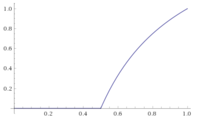
    Thus when p is 50% (or lower), \(Q=0\) and the lineage will die out. At any higher probability, \(Q\) is nonzero and becomes progressively higher until it reaches \(Q=1\) when p = 100%.

    The simple functional equation arose from the self-similar infinities involved—there are no edge cases when there are no edges. This puzzle is an instance of percolation.

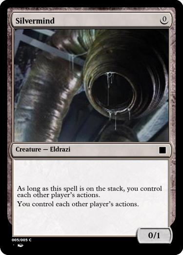
30. Magic duel. To find out whether Magic: The Gathering is geared toward attack or defense, imagine the following scenario. You, playing defense, would like to successfully summon a creature. Your opponent would like to thwart you. If you both can invent any card abilities you like (subject to some fine print), who will succeed?

    Small print: You have priority. Invented cards must use existing mechanisms and language, not invent new concepts out of whole cloth.

    My solution, an irrefutable defender.

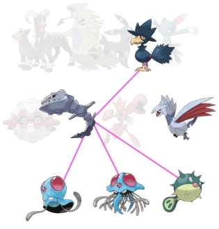
31. Pokémon linear optimization. The Pokémon type effectiveness chart can be represented as a matrix \(\mathbf{S}\), with one row and column for each type. Type effectiveness is either 2x, 1x, 0.5x, or 0x, but if you use the log of the effectiveness values instead (respectively +1, 0, -1, -∞), you can use matrix multiplication to compute the vulnerabilities of any type combination.

    For example, if \(\vec{t}\) is a column vector with a 1 in the Grass and Poison positions and 0 elsewhere, then \(\mathbf{S}\vec{t}\) will be a vector listing the susceptibility of a Grass-Poison type to each attack type.

    You can use the matrix approach to ask and answer questions about type effectiveness. For example, if you can combine more than two types, can you make a type combo that is resistant to every type? (Find \(\vec{u}\) so that \(\mathbf{S}\vec{u} \leq \vec{0}\).) Yes. In Gen II onward¹⁰, that type combo \(\vec{u}\) is

    {:ground 1,
     :poison 2,
     :flying 1,
     :dark 1,
     :steel 1,
     :water 2}.
    

    This combination uses eight types, which is minimal. There is exactly one other minimal solution (Challenge to the reader: can you find the other minimal solution?)

    Side challenge: Assemble a team of four pokemon such that each of these eight types is represented. (For example, a Nidoking would take care of Ground and one Poison; a Zubat would take care of Flying and the second Poison.) Answer in footnote¹¹.

32. Magic Squares. I once saw a 4x4 magic square, where the magic sum appeared not only in the rows, columns, and diagonals, but also the four corners, the 2x2 corner squares, the central 2x2, and opposite pairs of "incisors" in between the corner squares.

    \(\begin{bmatrix} 17 & 10 & 7 & 17 \\ 20 & 4 & 21 & 6 \\ 5 & 11 & 15 & 20 \\ 9 & 26 & 8 & 8 \end{bmatrix}\)

    I wondered how many free parameters such a magic square had. There are 16 variables (4x4 entries) and 18 different groups that sum to the same magic number. The linear sum constraints¹² form an 18x16 matrix, whose null space has exactly 6 rows, meaning it takes exactly six independent numbers to specify all the entries completely.

    The acutal required number is seven: the null space method assumes all the groups sum to zero. The seventh parameter is your chosen value of the magic sum.

    import numpy as np
    import scipy.linalg
    
    # A B C D
    # E F G H
    # I J K L
    # M N O P
    
    A,B,C,D,E,F,G,H,I,J,K,L,M,N,O,P = np.identity(16)
    
    # WHICH THINGS SUM TO THE MAGIC NUMBER?
    constraints = np.array([ A+B+C+D, # rows
                             E+F+G+H,
                             I+J+K+L,
                             M+N+O+P,
    
                             A+E+I+M, # cols
                             B+F+J+N,
                             C+G+K+O,
                             D+H+L+P,
    
                             A+F+K+P, # diagonals
                             D+G+J+M,
    
                             A+B+E+F, # corner 2x2
                             C+D+G+H,
                             I+J+M+N,
                             K+L+O+P,
    
                             F+G+J+K, # middle 2x2
    
                             B+C+N+O, # "incisors"
                             E+H+I+L,
    
                             A+D+M+P # corners
                             ])
    
                             Z = scipy.linalg.null_space(constraints)
                             print(Z.shape) # returns: (16, 6)
    

33. Mana polynomials. You can represent costs in Magic: The Gathering as polynomials in the mana symbols WUBRGC, with boolean coefficients.
    • Multiplication combines costs together. For example, R*R*R must be paid with three R.
    • Exponentiation is shorthand for repeated multiplication; exponents tell you how much of each color is required. For example, R¹U² represents the cost RUU.
    • Addition creates alternative costs. For example, (R+G) can be paid with R or G. As another example, (U+U+U) is redundant, equivalent to just U.
    • (!) Just like with numbers, you can distribute multiplication across addition. For example, (R+G)(R+U) = RR+RU+GR+GU. The two costs are equivalent to each other.
    • The "mana of any color" symbol is just (W+U+B+R+G+C).
    • The coefficients aren't numbers; they're boolean values ⊥ and ⊤. ⊥ is unpayable (multiplies like zero), and ⊤ is free-of-charge (multiplies like 1). Based on the meaning of addition and multiplication, we must also have ⊤+⊤=⊤, ⊥+⊥=⊥.
      • For example, R(⊤ + G) = R⊤ + RG = R+RG.
      • For example, R(⊥ + G) = R⊥ + RG = ⊥ + RG = RG.
      • For example, U+U+U = ⊤U+⊤U+⊤U = (⊤+⊤+⊤)U = ⊤U = U. (Redundant alternative costs become absorbed; coefficients are never higher than one and never negative.)
    • Mana polynomials have no nontrivial roots, basically because no combination of costs is unpayable ⊥ except the unpayable cost ⊥ itself.
    • A mana pool can be thought of as a monomial in this system (i.e. a polynomial with a single term like W³UUG); a pool exactly pays for a cost if the monomial appears in the polynomial. A simple formula is that the pool \(p\) exactly pays the cost \(c\) when \(p+c = c\). For example, as expected, an unpayable cost \(c=\bot\) is zero-like and never has this property; and an empty mana pool \(p=W^0U^0B^0R^0G^0C^0\) pays only for the gratis cost \(c=\top\).
    • There are no fractions or negative numbers in this system, but if there were, the wildcard cost X would have the formal value \[\frac{⊤}{⊤-(W+U+B+R+G)}\] because it is defined by the equation X = ⊤+(W+U+B+R+G) X.

34. Commuting polynomial chains. Two polynomials \(P(x)\) and \(Q(x)\) commute whenever \(P(Q(x)) = Q(P(x))\). Some polynmoials commute, and others don't. The set of powers \(\{x^1, x^2, x^3, \ldots, \}\) is an example of a chain—a list of polynomials, one of each degree, which all commute with each other. Are there any other chains?

    Any linear polynomial \(\lambda(x)=ax+b\), (where a is nonzero), has an inverse \(\lambda^{-1}(y)=(y-b)/a\). And if \(\{P_i(x)\}\) is a chain, then \(\{\lambda^{-1}\circ P_i \circ \lambda\}\) is also a chain. So every chain is part of a family of similar polynomials. Up to similarity, there is only one other polynomial chain: the Chebyshev polynomials \(T_n(x) \equiv \cos(n\cdot \cos^{-1}(x))\).

    Why? You can prove that any quadratic polynomials commutes with at most one polynomial of each degree (so the quadratic determines the whole chain), and each quadratic is similar to a quadratic of the form \(x^2+c\). In chains, the commuting constraint forces \(c(c+2)=0\). When \(c=0\), you get the power polynomials. When \(c=-2\), you get the Chebyshev polynomials. ref 1 ref 2.

35. Wrońskian derivative rules. The Wrońskian determinant satisfies several neat rules similar to the rules for derivatives:

    \[\begin{align*}W[f_1 \cdot g, \ldots, f_n \cdot g](x) &= g^n \cdot W[f_1,\ldots,f_n](x)\\ W[f_1 / g, \ldots, f_n / g](x) &= g^{-n} \cdot W[f_1,\ldots,f_n](x)\\ W[f_1 \circ g, \ldots, f_n \circ g](x) &= (g^\prime)^{n(n-1)/2} \cdot W[f_1,\ldots,f_n]\circ g(x)\end{align*}\]

    You can prove this by examining the pattern of derivatives, coefficients, and exponents you get when taking repeated derivatives of \(D_k(f\cdot g)\) or \(D_k(f / g)\) or \(D_k(f \circ g)\). In each case, they're linear combinations of the derivatives of \(f\) alone; the coefficients are polynomials in \(g,g^\prime, g^{\prime\prime}, \ldots, g^{(k)}\).

    For the product rule, the pattern comes from Pascal's triangle. For the chain rule, the pattern comes from the combinatorics of partitions, specifically the partition (Bell) polynomials. Arrange the \(g,g^\prime,g^{\prime\prime},\ldots\) terms into a matrix \(\mathbf{G}\) so you can concisely write, say, \(W[f_1\cdot g, \ldots, f_n\cdot g] = \text{det}\mathbf{G} \cdot W[f_1,\ldots,f_n]\). But \(\mathbf{G}\) is a triangular matrix in each case, so its determinant is the product of its diagonal entries. You can find those entries by following the pattern; this establishes the result.

36. Jacobian derivative rules. The Jacobian determinant \(\partial(f,g)\) of two functions \(f(x,y)\) and \(g(x,y)\) is the determinant of the matrix containing the single-variable partial derivatives of \(f\) and \(g\). Like the Wrońskian mentioned earlier, it is a derivative-based quantity. You can show that the Jacobian determinant follows product, quotient, and chain rules that resemble the rules for ordinary derivatives:

    \[\partial(f/g, h) = \frac{g \; \partial(f,h) - f\;\partial(g,h)}{g^2}\] \[\partial(fg, h) = f \; \partial(g,h) + g\;\partial(f,h)\] \[\partial(f\circ g, h) = (Df \circ g)\; \partial(g,h)\]

37. Pathfinding matrices. Given a directed graph with \(n\) nodes, you can build an \(n\times n\) adjacency matrix \(A\), where each entry \(A_{i,j}\) is one or zero, depending on if there's an edge \(i\rightarrow j\) or not. Surprisingly, you can use this matrix to count paths in the graph: you can prove that the matrix product \(A^p\) is a matrix whose \((i,j)\) entry is the number of paths between nodes \(i\) and \(j\) that have exactly \(p\) steps in the path.

    Or, if the edges represent distances, build a distance matrix \(D\), where each entry \(D_{i,j}\) is the length of the edge between \(i\rightarrow j\) (or \(\infty\) if there is no edge.) With a slight modification, we can use the matrix powers \(D^p\) to compute the shortest path between any two nodes. Just redefine arithmetic operations so that addition of two numbers instead computes their minimum, and multiplication of two numbers instead computes their sum. Then the matrix product \(D^p\) is a matrix whose \((i,j)\) entry is the length of the shortest route between \(i\) and \(j\) that has exactly \(p\) steps in the path.

38. Love triangles require same-gender attraction. Assume reductively that there are two genders. If we draw a diagram using dots (people) linked by arrows (attraction), a love triangle obviously requires three people and three arrows—where in any pair of people, one of them is attracted to the other.

    No matter which way the arrows are facing, your love triangle will always have a pattern of the form "A likes B and B likes C".

    If that pattern contains same-gender attraction, we're already done. Otherwise, the pattern implies that A and C are the same gender; hence the arrow between A and C (or vice-versa) constitutes same-gender attraction, and we're done in this case, too.

39. Efficient roll call in MTG. Each species of creature in Magic: The Gathering has a certain set of roles they can fulfill. One species might be able to fulfill only the Cleric role; one might be able to fulfill either the Cleric or Rogue role; and one might not be able to fulfill any role.

    An assignment assigns each creature to at most one of the roles it's capable of fulfilling. For a given set of creatures, your party size is the greatest number of distinct roles you can possibly assign, i.e. it's the number of distinct roles you fulfill when your assignment maximizes the number of distinct roles.

    I wondered how computationally difficult party size is in the abstract case: suppose you have k roles, and n creatures each capable of satisfying some (possibly empty) subset of those roles. How can you compute the party size?

    I was delighted to notice that this is a maximal matching problem on a bipartite graph: make a bipartite graph where one side contains a node for every creature, and the other side contains a node for each distinct role; wherever a creature can satisfy a role, make a link between them. In a bipartite graph, a maximal matching can be found efficiently: You treat it as a network flow problem and solve it (in polynomial time) using the greedy Ford-Fulkerson algorithm. The party size emerges as the maximum flow rate of the network.

40. Not Fibonacci! Can you find a set of numbers where the sum of any two distinct elements is unique? For example, the set {2,7,11} has this property because each sum (such as 13=2+11) can be uniquely decomposed—you can uniquely infer what the summands were.

    You can make an infinitely long sequence with this property. The smallest¹³ such sequence seems to follow a familiar pattern:

    1, 2, 3, 5, 8, 13, 21, 30, 39, 53, …

    Strangely, this sequence isn't the Fibonacci sequence—it just happens to agree with it for seven terms. I am not sure why. The Fibonacci sequence does seem to satisfy the "distinct sum" property; it's just not the minimal sequence that does.

    (Originally, I wanted to make a symbolic nomogram where instead of addition of numbers, I had combination of discrete symbols. To do so, you need a way to map symbols covertly onto numbers.)

41. Diverse denominations. Here's a numismatic problem: you want to assemble a collection of coins that can be variously combined to make any integer amount of money between (say) $1 and $100. You may choose coin denominations of any integer amount (e.g. you can have a $3 coin if you want), and you can have multiples of the same denomination (e.g. multiple $4 coins). One allowable, if extreme, solution would be to have a collection of 100 coins for $1 each. Find a solution that uses as few coins as possible.

    (Example: In a simpler version of this problem, you need to make any integer amount of money between $1 and $10. You can do so using the collection of coins [$1, $2, $2, $5].)

    Answer: (hidden in footnote) ¹⁴

42. Yarn counting. Every planar graph gives rise to an alternating knotwork, as discussed here. The knotwork is a tangle of some number of separate threads. To count the number of threads, you can use the formula: \[|T(-1,-1)| = 2^{c-1}\]

    Where T is the Tutte polynomial of the planar graph, and c is the number of threads. Because the Tutte polynomial is a graph invariant, the number of threads stays the same no matter how the graph is drawn/embedded.

43. Disintegrating water. (The sea of Theseus) Very rarely, a water molecule can tear apart into a proton and hydroxide ion. For this process, a water molecule has a half-life of around 7.7 hours. Based on that figure, you can calculate how long it would take to be 99% certain that every molecule of water in some container had disintegrated at least once. For 1mL of water, it comes out to around 26 days. Every time you double the amount of water, you (basically) add another half life to the total. For a human body with 50L of water, it takes around a month—31.1 days for all the water to turn over. Amazing!